Sunday, December 12, 2010

How long is the period of random numbers created by java.util.Random?

The answer is, pretty darn long! 


I feel a bit cheated for not knowning, while I had several times seen the code the years before.


So it uses a good old linear congruential generator:


x = A * x + C


So, java.util.Random uses these two constants (A and C respectively):


    private final static long multiplier = 0x5DEECE66DL;
    private final static long addend = 0xBL;

Quite appropriate to place two "random" numbers in the Random class, right? Only these are not entirely random...

0x5DEECE66DL % 8 == 5
and 
0xBL is an odd.

So what? 


It turns out, when these exact conditions are satisfied, the defined period is maximal, so the generated period (x is long) is 2^64. This piece of magic is documented here, page 9. The "why" of it is beyond me. 

If any ninja mathematician comes across this post, please leave some explanation if you can.


EDIT: oops. I overlooked that java.util.Random uses a mask to only reduce itself to 48 bits, instead of 64, so correspondingly the period is 2^48 instead of 2^64; apparently in an attempt to increase the quality of the generated numbers. In any case, if you need longer period, the technique described here will do the trick.

Juggling consistent hashing, hashtables, and good old sorting

Consistent hashing can be summarized in one sentence: it is a hashtable with variant-length buckets.

You have a line segment (that's the key space). Breaking it to N equal parts (the buckets) means it is very easy (O(1)) to compute which part contains a given point. But if you increase or decrease N, all parts change (and shrink or grow respectively). Only the first and the last part have one of its ends unaffected, but the rest have both their ends moved.

Now consider breaking it in N parts, but not of necessarily the same length. Now it is easier to change the number of parts. Do you want more parts? Break one in two pieces. Want fewer parts? Merge two parts sitting next to each other. All other parts remain firm in their place, unaffected. But now finding which part contains a given point gets more complicated (O(logN) if you keep the parts sorted, say in a red-black tree).

Hashtables themselves can be summarized in an interesting way: it is sorting...by hash (it doesn't matter if the original key space is not totally ordered - the hashes are). But if it is sorting, where the logN factor in the complexity of hashtable operations? Well, there isn't one: hashes are small natural numbers (bounded by the hashtable size, which is O(N) of the elements in it). And what do you think of when you want to sort small natural numbers? Counting sort. (Caveat: hash functions do not just aim to map a large key space into a sequence of natural numbers, that's only part of the story. They also aim to approximate a random permutation of the original space, which is separately useful - to try to load balance the buckets when the incoming distribution is not uniform. In consistent hashing, we sacrifice the first role of hash functions, but we keep this latter one).

Trying to compress the discussion above:

  • Hashtables are really counting sort
    • (Yes, data structures are algorithms)
    • An equal piece of the (approximately permuted) key space is mapped to each bucket
      • Easy to find the corresponding bucket for a key (++)
      • Changing the number of buckets affects the mapped spaces of all buckets (--)
  • Consistent hashing differs in the following way:
    •  A variable piece the (approximately permuted) key space is mapped to each bucket
      • Harder to find the corresponding bucket for a key (--)
      • Easy to split or merge buckets, without affecting any other buckets (++)


Bonus section: Bigtables (and the good old Bigtable paper here). In Bigtable, The rows are primarily sorted by row key. The tablets (think buckets) are variable length, so that overloaded tablets can be split, without touching the huge amount of data that potentially reside in the same bigtable. (One can help load balancing the tablets by -did you guess it?- sorting by hash first...). So, here you go. The rows are sorted. Yet it can still rightfully be described as consistent hashing. Confused yet? Well, at least I tried. :)

Wednesday, October 20, 2010

Memory cost (per entry) for various Java data structures

Have you seen this? http://code.google.com/p/memory-measurer/wiki/ElementCostInDataStructures
It shows the memory cost per each entry for various common and not-so-common Java data structures. For example, have you wondered when you put() an entry to a HashMap, how much memory footprint you create, apart from the space occupied by your key and your value (i.e. only by internal artifacts introduced by HashMap itself)? There are the answers to such questions.

It also exemplifies the utility of my memory measuring tool, which I recently redesigned to decouple object exploration from measuring the memory usage (bytes) of objects, so I can use the same exploration to derive more qualitative statistics, like number of objects in a object graph, number of references, and number of primitives (which would directly reflect memory usage if it weren't for effects of alignment).

If you are designing data structures in Java, it would be silly not to use this tool. Seriously. (Profilers can be used to somewhat the same effect, but why fire it up and click buttons till you get where you want and take numbers and calculate by yourself, when you can do it more precisely with very simple code).

Future work: do the same for the immutable Guava collections.

Thursday, July 29, 2010

Graph reachability, transitive closures, and a nasty historical accident in the pre-google era

Last few days I'm feeling a bit like an archaeologist. It's probably a great story to explain to a newcomer just what's the importance of the internet, coupled with a great search engine. But I digress.

What follows is a pretty long post, covering a lot of ground in the graph reachability problem and transitive closures, enumerating various naive solutions (i.e., the ones you are likely to see used), then moving to much more promising approaches.


Introduction


Let's say you have a directed graph, G = (V, E), and you want to know real fast whether you can reach some node from some other, in other words whether there is a directed path u --> v, for any nodes u and v. (Take a moment to convince yourself that this is a trivial problem if the graph is undirected). Before we continue, lets stop and think where this might be useful. Consider a (really silly) class hierarchy (we also call it an ontology):


Testing whether there is a directed path between two nodes in a class hierarchy is equivalent to asking "is this class a subclass of another?". That's basically what the instanceof Java operator does (if we only consider classes, then subtyping in Java forms a tree - single inheritance, remember? - but if we add interfaces in the mix, we get a DAG, but thankfully, never a cycle).

Lets formally denote such a query by a function existsPath: V x V --> {1, 0}. It takes an ordered pair of nodes, and returns whether there is a path from the first to the second. Now, lets make sure that having such an existsPath function is, in fact, the characteristic function of the transitive closure of the graph, that is, given any edge, we can apply this function to it to test whether it belongs to the transitive closure or not, i.e., whether it is one of the following edges:


When we talk about transitive closure, though, we mean something more than merely being able to answer graph reachability queries - we also imply that we possess a function successorSet: V --> Powerset(V). i.e., that we can find all ancestors of a node, instead of checking if a particular node is an ancestor of it or not.

By the way, the above explanation is exactly the reason why in Flexigraph I define the interfaces (sorry, but blogger doesn't play very nicely with source code):


public interface PathFinder {
    boolean pathExists(Node n1, Node n2);
}

public interface Closure extends PathFindr {
    SuccessorSet successorsOf(Node node);
}

"Closure extends PathFinder" is basically a theorem expressed in code, that any transitive closure representation is also a graph reachability representation. That's the precise relation between these two concepts - I'm not aware of any Java graph library that gets these right. Continuing the self-plug, if you need to work with transitive closures/reductions, you might find the whole transitivity package interesting - compare this, for example, with JGraphT support, or yWorks support: a sad state of affairs. But I digress again.

Supporting graph reachability queries

Ok, lets concentrate now on actually implementing support for graph reachability queries. These are the most important questions to ask before we start:
  • How much memory are we willing to spend?
  • Is the graph static? Or update operation are supported (and which)?
Lets explore the design space based on some typical answers to the above questions.

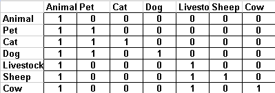
Bit-matrix: The fastest reachability test is offered by the bit-matrix method: make a |V| x |V| matrix, and store in each cell whether there is a path from the row-node to the column-node. This actually materializes the transitive closure, in the sense that we explicitly (rather than implicitly, to some degree) represent it (and we already argued that representing the transitive closure also implies support for graph reachability queries).


Of course, this has some obvious shortcomings. Firstly, it uses O(|V| ^ 2) memory - but this is not as bad as it looks, and it would probably be a good solution for you if your graph is static. Which leads us to the second problem - it is terrible if you expect to frequently update your graph.

Adjacency-list graph representation: another way of representing the transitive closure is to just create an adjacency-list graph with all the edges of the transitive closure in it. In the example, that would mean to create a graph to represent the second image. (This is what JGraphT and yWorks offer - it's the simplest to implement). This has numerous disadvantages. First, this is a costly representation - such a representation is good for sparse graphs, but it is very easy for a sparse graph to have a dense transitive closure (consider a single path). Worse, if you represent each edge with an actual "Edge" object, then you are quite probably end up with a representation even costlier than the naive bitmap method - compare using a single bit to encode an edge vs using at least 12 bytes (at least, but typically quite more than that), i.e. 96bits. Also, this representation doesn't even offer fast reachability test - testing whether two nodes are connected depends on the minimum degree of those nodes, and this degree can be large in a dense graph. All in all, this representation is the lest likely to be the best for a given application.

Agrawal et al: Now, lets see the approach in a very influential paper published in 1989:  Efficient Management of Transitive Relationships in Large Data and Knowledge Bases. Lets see a figure from this paper, starting from the simple case of supporting reachability queries in a tree


(Don't be confused by the edge directions, they just happened to drew them the other way around). Each node is labelled with a pair of integers - think of each pair as an interval in the X-axis. The second number is the post-order index of that node in the tree, while the first number is equal to the minimum post-order index of any descendant of that node. Lets quickly visualize those pairs as intervals:


As you can see, the interval of each node subsumes (is a proper superset of) the intervals of exactly its descendants. Thus, we can quickly test whether "e is a descendant of b" by asking "is 3 contained in the interval [1, 4]?", in O(1) time. 


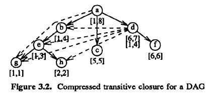
Quick check: does it easily support graph updates? No! Inserting a new leaf under node g would require changing the numbers of g and everything on its right (that is, all the nodes of the graph!). And we are still only discussing about trees. Lets see how this generalizes for acyclic graphs (this can be similarly generalized to general graphs, but I won't elaborate on that here). Again, a figure from the paper:


Note that some non-tree edges have been added, particularly d --> b (the rest of the inserted are actually redundant, yes, they could have used a better example). Also note that now d is represented by two intervals, [6,7] and [1,4]. The same invariants are observed as above - the interval set of each node subsumes any interval of exactly its descendants. Basically, we start with a tree (forest) of the graph, label it as previously, and then process all non-tree edges, by propagating all the intervals of the descendant to all its ancestors via that edge.


Second check: how does this cope with graph updates? Much worse! If, for example, we have to change the interval of g, we now must search potentially the whole graph and track where its interval might have been propagated, fixing all those occurrences with the new interval of g. Well, this sucks big time.


Now, lets try to justify the "historical accident" that the title promises. What if I told you that this problem was already solved 7 years earlier than Agrawal reintroduced it? More importantly, what if I told you that (apparently!) hardly anyone noticed this since then? It's hard to believe. For example, here is a technical report published recently, in 2006: Preuveneers, Berbers - Prime Numbers Considered Useful . Don't bother reading all those 50 pages - here is a relevant quote (shortly after having presented the Agrawal et al method - emphasis mine):


In the previous section several encoding algorithms for efficient subsumption or subtype testing were discussed. As previously outlined, the major concern is support for efficient incremental and conflict-free encoding. While most algorithms provide a way to encode new classes without re-encoding the whole hierarchy, they often  require going through the hierarchy to find and modify any conflicting codes. The only algorithm that does not suffer from this issue is the binary matrix method, but this method is the most expensive one with respect to the encoding length as no compaction of the representation is achieved.
This statement is the authors' motivation for design a new approach (a not too practical dare I say, requiring expensive computations on very large integers). They didn't know the solution.

Here is another example, published in 2004.Christophides - Optimizing Taxonomic Semantic Web Queries Using Labeling Schemes. This is a great informative paper surveying at depth a number of different graph reachability schemes, with a focus on databases. Christophides, actually, is my former supervisor, Professor at the University of Crete, and a good friend. Unfortunately, even though this paper actually cites the paper that contains the key idea, they also didn't know the solution (this I know first-hand).

Yet another example, published in 1999: Bommel, Beck - Incremental Encoding of Multiple Inheritance Hierarchies. Again, they didn't know the solution, so they ended up creating a more complicated, less-than-ideal work-around (see for yourself).

I don't even dare to look into all ~250 papers that cite Agrawal's work.

This is rather embarrassing. Before continuing, this kind of regression would have been highly unlikely if there was an efficient way (e.g. google scholar :) ) to search for relevant research. Here goes the obligatory memex link.

That being said, lets finally turn our attention to the mysterious solution that was missed by seemingly everyone. Dietz - Maintaining order in a linked list. This paper was published much earlier - in 1982, a year special to me since that's when I was born. Dietz introduces the (lets call it so) order maintainance structure, defined by this interface:
  • Insert(x, y)
    Inserts element x right afterwards element y.
  • Delete(x)  (Obvious)
  • Order(x, y) 
    Returns whether x precedes y.
So this is basically similar to a linked list, with the addition that we can ask (in constant time!) whether a particular list node precedes another. The actual data structure proposed to fulfill this interface has been superseded by Dietz and Sleator in Two Algorithms for Maintaining Order in a List (1988), and then recently by Bender et al in Two Simplified Algorithms for Maintaining Order in a List. These structures offer amortized O(1) time complexity for all these operations (there are also versions offering O(1) worst case, but they are significantly more complex to implement, and likely to be slower in practice). Here is my implementation of Bender's structure.


So how can this structure solve the incremental updates problem? Let's see Dietz' solution of the case of trees. Lets draw another tree.


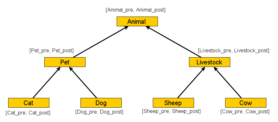
Okay, so this is the same tree, and I have labelled the nodes with intervals, with one catch - the intervals do not comprise integers, but symbolic names. What's the deal, you say? Here's the deal!


That's it! The colors are there so you can easily match-up the respective nodes. This is a linked list, or more precisely, the order-maintainance list. Any two nodes in it define an interval. For example, [Pet_pre, Pet_post] interval (green in the picture) subsumes both Cat's and Dog's nodes - precisely because it is an ancestor of both! Note that, internally, these list nodes do in fact contain integers that observe the total order (e.g., are monotonically increasing from left to right) so we can test in O(1) whether a node precedes another. This is quite a simple structure, and there are very good algorithms for inserting a node in it - if there is no space between the integers of the adjacent nodes, an appropriate region of this list is renumbered.


Update: probably it's obvious, but better be specific. So how do we add a descendant? Let's say we want to add a graph node X that is a subclass of Pet. We simply create two list nodes, X_pre, X_post, and insert them right before Pet_post. That would result in a chain Pet_pre --> [whatever nodes were already here] --> X_pre --> X_post --> Pet_postOr we could add these right after Pet_pre, it's equivalent really. (As a coincidence, both Dietz and I chose the first alternative, to insert child_pre and child_post right before parent_post. I had a reason for this actually, there is a tiny difference because I'm using Integer.MIN_VALUE as a sentinel value, but that would be way too much details for this post). Of course, to insert a node, say B, between two others, say A and C, we have to find an integer between label(A) and label(C), i.e. to make sure that we have label(A) < label(B) < label(C), without affecting any existing label relation. If label(A) = label(C) + 1 (i.e., consecutive, no space between them for a new node), we have some nodes to make space at the place of insertion. Compare with Dietz' Figure 4.1, in the "Maintaining order in a linked list" paper.


While this might not seem such a big win for the case of trees, it is absolutely necessary in the case of graphs. This is what Agrawal et al missed! Instead of using integers directly, they should have used nodes of an order-maintainance structure. Why? Because when an interval does not have space to accommodate a new descendant, instead of widening the interval and then scanning the whole graph to find appearances of those integers to fix them, we instead make only local changes in the order maintainance structure in O(1), without even touching the graph!


You can visualize the difference in the following example.
The segmented edges are non-tree edges, so they propagate upwards the intervals, thus, the H node ends up having 4 distinct intervals. Now, if instead of nodes such as E_pre and E_post, we had numbers (say, (5,6)), what would have happened if we wanted to add a descendant under E but it had no space in its interval? We would fix the boundaries of E's interval, and we would have to search the graph to see where the old boundaries have been propagated (i.e. in nodes F and H). With the order maintainance structure, this is not needed. We locally renumber whichever node is required, and we do it once - we only renumber E_pre and E_post once, and due to node sharing (instead of copied values/integers!), it doesn't matter where these might have been propagated, all positions are automatically fixed too! Contrast this to having to visit F, G and H, find E_pre, E_post in their intervals, and fix them in all places. Let alone if we had to renumber a series of intervals, and hunt the propagations of all of them in the graph, and so on...


Just for completeness, this is what the order maintainance list would look like, in the last example:


A_pre --> B_pre --> C_pre --> D_pre --> E_pre --> E_post --> D_post --> F_pre --> F_post --> C_post --> G_pre --> G_post --> B_post --> H_pre --> H_post --> A_post.


In this structure we perform the renumbering, not in the graph! Particularly, in some (typically small) region that contains the two nodes inside which we want to insert something.


So, there you go. This is the trick I (re)discovered on some Friday of last March, and ended up coding  http://code.google.com/p/transitivity-utils in the following weekend, which implements all of the above and more, so you don't have to. It is hard to believe that this went unnoticed for 20 years - and even harder to believe that the solution was there all along, waiting for someone to make the connection. 


Now that's something to ponder about. Oh, and thanks, Dietz, great work!


If you managed to read all the way down to here, my thanks for your patience. That was way too long a post, but hopefully, you also earned something out of it. I regard this a very interesting story, and wish I was a better storyteller than this, but here you go. :)

Sunday, July 25, 2010

Google File System - the 'bandwidth' problem

I am reading the very interesting Google File System paper. It describes the situation back in 2003, not sure how much things have changed since then. Before moving to the subject of this post, lets sum up some interesting points of that paper first (only based on my certainly incomplete understanding).


  • GFS clearly favors appending to files than random access writing. If all mutations of a file are appends, sequential readers (readers that scan the whole of the file - which represents the vast majority of cases) have also extra consistency guarantees: in the face of concurrent modifications, the only "bad" thing that they may see is the file ending prematurely. But everything up to that point is guaranteed to be well defined and consistent.
  • A GFS file can be used as an excellent producer-consumer queue! Multiple producers may append ("record append") to the file, with no need for extra synchronization/distributed locking. This is a weaker form of append - the client does not choose where the data end up to, the primary replica server of that file chooses this, and the clients get a guarantee that the update with occur at least once (well, not exactly once, but one can work-around this by uniquely naming the records, if they aren't already named so). This seems much simpler and better than either having to establish distributed locking protocols between producers, or letting them choose the offset in the file where their append should take place, and trying to resolve potential (and possibly very frequent) collisions.
  • Automatic garbage collection of orphaned chunks (file pieces) is implemented.
  • There are quite weak concurrency guarantees for writers that write lots of data. The writer client needs to break up the data into acceptably small pieces, and each piece is written atomically - but if there are multiple writers doing the same, the final result is undefined, it could contain random fragments of the data of each writer.
  • File metadata updates are atomic. This is particularly nice, consider the following case: a writer writes to a file, and after  it's done writing, it atomically renames the file to a name which can then publish to readers. This is the analog of doing a compare-and-swap (CAS) in a shared memory multiprocessor (SMP), which, importantly, is the base of most lock-free algorithms. In particular, the writer that writes to a file (unknown to others) is like a thread doing thread-local computation, and only announce the result in the end via an atomic pointer update (atomically update a root pointer, if nobody has already changed it, or in GFS, if nobody has created the intended filename first).
Now, on to the piece that found curious enough to make a post about. A couple of key points:
  • When a client wants to write, it can pick whatever replica to initiate this action (presumably the replica closer to it - and in Google's case, they can infer the "closeness" of two nodes by inspecting their IPs). 
  • The data must be stored (temporarily) to all replicas before the client notifies the (designated) primary replica that the write should be committed. 

This leads to the problem: How to move client's data to be written, to all replicas? Google's answer is through a chain (hamiltonian path) through all replicas, starting at the replica that was contacted by the client. This is preferred over e.g. a dissemination tree, so as to bound the requirements of out-bandwidth of  replicas - perhaps the best dissemination could be a star-like tree, but too much burden would be placed on the central node, and so on). 

Here is a picture taken from the aforementioned paper. Note the thick arrows, they show the chain that data goes through, from the client and to all replicas. 
But how do we choose the next replica in the chain? I.e., why we send the data from Replica A to the Primary Replica and then to Replica B, rather than the other way around? Google is using a simple, greedy rule: pick the replica (that hasn't seen the data yet) that is closest to the current one.

This looks like the well (ok, perhaps not so well) known graph theoretic problem, the Bandwidth Problem. That is, we have a graph, and we want to create some linear order of the nodes, so that we minimize the total edge distances (e.g. if we put nodes side-by-side, the edges between them would have very low distance/cost). It's NP-Hard.

To visualize the bandwidth problem, I'm stealing a picture from the excellent Skiena's book, the Algorithm Design Manual, which I highly recommend. (I guess a free ad here should worth stealing a small picture :-/ ). (By the way, here is an excellent treatment of the problem by Uriel Feige, very conveniently containing approximation algorithms and heuristics).


Well, almost, but not exactly the same problem. The subtle difference is that in the Bandwidth Problem, we seek to minimize the distance/cost sum of all edges, while in the case of GFS, we only need to minimize the length of a single (any) Hamiltonian path (the picture just shows an easy case, where apart from a single path there are no more edges in the graph).

Ok, so I don't know yet how to state this problem. (While reading the paper, I thought it was the same problem, thus the title of this post). Let me do something else for now - lets try to be create an example that maximizes the cost for GFS' heuristic. Here is what I came up with (click to see larger size):


I think that's the worst case scenario. The client chooses the replica in the middle, then we go to the right 1 step (because the one at the left is at distance 2), then we go to the left 3 steps (because the one at the right is at distance 4), and so on, going back and forth, with a total distance travelled = 1 + 3 + 7 + 15 = (2^1 - 1) + (2^2 - 1) + (2^3 - 1) + (2^4 - 1) = (2^5 - 1) = 31, or more generally, exactly 2^N - 1! (Of course, don't hold your breath on ever seeing such a topology in an actual GFS cluster!) The optimal solution here would be to go immediately to a boundary replica, either farthest left or right (choose the one closest), and then linearly visit the rest. That would yield a cost of (1 + 4) + (1 + 2 + 4 + 8) = 20, (1 + 4 to go to the farthest right replica, and then going all the way to the left) or more generally, exactly 2^(N - 1) + 2^(N - 3) (it's fun to work this formula out!). 

Now, how much worse is Google's heuristic than the optimal solution? 

It turns out, (if we assume that I did find the worst case scenario)Google's solution is at most a factor of 8/5 (= 1.6) of the optimal solution! (Well, sure enough. To compare 2^N to 2^(N-1) + 2^(N-3), divide everything by 2^N, so we have 1 compared to 1/2 + 1/8, or 5/8). Wow! That's extremely good for something as simple! I didn't expect to find such an exact result - one can also compute this easily via WolframAlpha, which is way too cool in this kind of problems.

Nice, nice, nice. I thought I would be find something ludicrously bad (in a completely unrealistic scenario), but it turns out, that's just 1.6 times the optimal solution at most!


/sheer happy - we haz it :)

Addendum:


Ah, the art of creating good corner case examples. It turns out the above is not the worst case, there is a worse than that, and quite simpler too (I had thought about this earlier, but for some reason I decided that forcing the algorithm to continually go back and forth would be the most expensive).

Consider this example (again, click to see in full size):

Each adjacent replica pair is separated by unit distance, while the last two are separated by two. We can make the path arbitrarily long, easily forcing the algorithm to choose a path which is a factor of 2 - ε longer than the optimal. And this is to be further restrained: I'm only considering geometric graphs, i.e. graphs where the triangle inequality holds. I have next to no idea whether actual network topologies resemble geometric graphs, and certainly one could construct much worse examples in graphs where the notion of distance is completely arbitrary (but distances in a network topology certainly isn't an arbitrary function). It's too late in the night to worry about that, so lets stop here hoping I'm still making some sense. :)

By the way, I recently bought Vazirani's Approximate Algorithms book. Neat, refreshing read, and highly recommended.

Monday, June 21, 2010

My oldies but goldies pet projects

Finally! I took the time to upload some of my old pet projects on google code. Briefly:


  • Flexigraph: a life-saver of a graph library. :) Packed with several unique features, but I have no time to comment them. Especially the Traverser API scoffs at all other java graph libraries of today (and this is several years old by now).
  • JBenchy: (my friends know this by the imaginative name "aggregator"). This is another life-saver if you are in the business of doing benchmarks/experiments and want a systematic way to store and analyze your collected points. Leverages the sheer expressive and analytical power of SQL GROUP BY statements, yet it hides all SQL from you so you can concentrate on your benchmark itself. It can also create nice diagrams for you, if you need some help with visualization.
  • MemoryMeasurer: Another uncharacteristically exotic name for a project! This little gem can compute the memory footprint of an arbitrary object graph / data structure. Did you ever wonder how much space does a default HashMap takes? Or an ArrayList of 5 HashMaps? Or whatever? Well, this is the tool for you. Also note that you can use it with JBenchy to create benchmarks for data structures, if this happens to be your thing. Oh, by the way, a new HashMap() takes 120 bytes, in case you did wonder.
Good! All my pets in line, with a new home. Enjoy :)

Thursday, May 6, 2010

Motivating Divide and Conquer paradigm

Just the other day I went in my old University, met former teachers and collaborators... fun!

I also attended a lecture on algorithms. The topic: Divide and Conquer.

The professor presented a very simple example to make the technique apparent. The problem? Find the minimum element of a list. Instead of doing the usual (in pseudocode):

result = +oo;
foreach e in list {
  result = min(e, result)
}

The divide 'n conquer approach would be:

function min(list)  {
  if (list.size == 1) return array[0]
  else {
    k = list.length / 2
    return min(
      findMin(list.subList(1, k)), 
      findMin(list.subList(k+1, list.size)))
  }
}

One could ask, "what's the point". In this example, this doesn't sound important at all. A student with good practical experience with programming would readily recognize that the latter, sophisticated approach is likely to perform worse than the straight-forward iteration. Indeed, a student there asked, "do we gain any gain in time complexity by following the latter approach in this example?". Unfortunately, the answer was no, both versions are O(n), so the exercise "is" pointless. 


Quite some years after the period when I was an undergraduate student, and reflecting on that experience, that was my main gripe with how Computer Science was being taught. Without proper motivation! The student must somehow "guess" by him/herself the importance of the covered topics. An example dialogue that could ensue between students: "-Hey, what did you learn today? -Nothing much, something called 'divide and conquer', it's just a way to create complicated solutions when simple and as good solutions already exist".


Since I was attending, I thought I should intervene and give the very, very, very imporant motivation for learning this algorithm design paradigm. The reason is the all-too-known fact that CPUs have stopped getting faster, and they only become more numerous. This can be easily recognized, but it also has a tremendous implication in how we design software. Even for this simplistic problem, the first method of computing the minimum element is doomed. It may not fail tomorrow, it might not fail next year or the year after, but it's doomed nevertheless. Imagine you have a billion elements of which to find the minimum. Also imagine your run-of-the-mill computer has hundreds of processing cores (by the way, we should stop calling them CPUs/Central Processing Units, how "central" is something you have hundreds of?).


Here is the expression that the first method is trying to evaluate:


I.e., you first find the minimum of the first two elements, then you find the minimum of that and the third element, then the minimum of that and the fourth element, etc, etc. The point is, the Kth call (K>1) to min() always must wait first for the result of the (K-1)th call of min() to become available. Each min() invocation takes (say) a unit of time, so the final computation cannot consume less that K time units, no matter whether you have a single core or thousands of them. The so called "critical path" (the longest path of things that must happen sequentially) as is also apparent in the diagram, has length K. Bad.

This is what happens with divide and conquer instead:


Still, the root depends to two other min() invocations, and must wait for them before evaluating itself. But those two are not dependent on each other, they may run in parallel. The critical path here has length only logK. Thus, divide and conquer can solve this problem in O(logN) instead of O(N). Without leaving your excess of processing cores to sit (and waste energy) idly.

As I explained to the student, this epitomizes programming of the future. Of course that's a hyperbole, but hyperboles are useful to drive a point home. And it is certainly better than present something dry to the student, without any hint of its importance - that's the recipy to make him/her not pay attention, and soon forget about this weird, exotic thingy.

That's all for now! Oh, and if you want to actually implement algorithms like this, and you code in Java, the fork/join framework is something you'll definitely want to learn.

Tuesday, April 13, 2010

My solution to Matrix-Chain-Order problem (Chapter 15 of CLRS)

For practice, I tried solving the problem "Matrix-Chain-Order" that appears on section 15.2 of Introduction to Algorithms (that's the chapter on Dynamic Programming). In short, one gets a list of (compatible) matrices, A1, A2, A3... An, and the problem is to compute the optimal order for creating their product. 


I liked my solution, so I'm posting this just for the record. This should be helpful if one is reading that section and looks for a Java implementation of that problem (in order to compare with his own solution of course :)). To make it tougher, I tried it writing this first on paper, then in my IDE, to see how many errors would slip in the paper version. There were two: a single off-by-one error in the inner loop (damn!), and that I forgot some components of the cost of a particular multiplication expression.


It creates optimal multiplication expressions of increasing width. Initially width == 1, and we just have the leaves, the matrixes themselves. Next, we find the optimal expressions of width == 2, but there is only one order to multiple 2 arrays, so nothing special happens. After that, things get more interesting, since we get to create various possible trees for each sequence of matrixes, and retain the best.


Amazingly, it is exactly one year (to the day!) ago that I posted a same exercise in tree building (enumerating binary trees, also via dynamic programming): http://code-o-matic.blogspot.com/2009/04/wonderful-programming-exercise.html
I think I need more diversity :)


Anyway. The main method is this:


    public static void main(String[] args) {
        Op op = matrixChainOrder(Arrays.asList(
                new Matrix(30, 35),
                new Matrix(35, 15),
                new Matrix(15, 5),
                new Matrix(5, 10),
                new Matrix(10, 20),
                new Matrix(20, 25)));
        System.out.println(op);
        System.out.println("Cost: " + op.cost());
    }

And it prints:

(([30 X 35] * ([35 X 15] * [15 X 5])) * (([5 X 10] * [10 X 20]) * [20 X 25]))
Cost: 15125

(This mimicks the example and solution of the book, but it also creates the expression of the multiplication, easy to pretty-print and ready to be computed).

The full code:

import java.util.*;

public class Matrixes {
    public static void main(String[] args) {
        Op op = matrixChainOrder(Arrays.asList(
                new Matrix(30, 35),
                new Matrix(35, 15),
                new Matrix(15, 5),
                new Matrix(5, 10),
                new Matrix(10, 20),
                new Matrix(20, 25)));
        System.out.println(op);
        System.out.println("Cost: " + op.cost());
    }

    static Op matrixChainOrder(List matrixes) {
        Map optima = new HashMap();
        for (int i = 0; i < matrixes.size(); i++) {
            optima.put(new Interval(i, i), new Leaf(matrixes.get(i)));
        }
        for (int width = 1; width < matrixes.size(); width++) {
            for (int offset = 0; offset < matrixes.size() - width; offset++) {
                Op best = DUMMY;
                for (int cut = 0; cut < width; cut++) {
                    Op left = optima.get(new Interval(offset, offset + cut));
                    Op right = optima.get(new Interval(offset + cut + 1, offset + width));
                    Op mul = new Mul(left, right);
                    if (mul.cost() < best.cost()) {
                        best = mul;
                    }
                }
                optima.put(new Interval(offset, offset + width), best);
            }
        }
        return optima.get(new Interval(0, matrixes.size() - 1));
    }
    private static final Op DUMMY = new Op() {
        public int cost() { return Integer.MAX_VALUE; }
        public Matrix compute() { throw new AssertionError(); }
        public int rows() { throw new AssertionError(); }
        public int columns() { throw new AssertionError(); }
    };

    private static class Interval {
        final int begin;
        final int end;
        Interval(int begin, int end) { this.begin = begin; this.end = end; }
        public boolean equals(Object o) {
            if (!(o instanceof Interval)) return false;
            Interval that = (Interval)o;
            return this.begin == that.begin && this.end == that.end;
        }
        public int hashCode() { return 31 * begin * (17 + end * 31); }
        public String toString() { return "[" + begin + ".." + end + "]"; }
    }
}

class Matrix {
    final int rows; final int columns;
    Matrix(int rows, int columns) { this.rows = rows; this.columns = columns; }
    int rows() { return rows; }
    int columns() { return columns; }
    public String toString() { return "[" + rows + " X " + columns + "]"; }
}

interface Op {
    int cost();
    Matrix compute();
    int rows();
    int columns();
}

class Leaf implements Op {
    final Matrix matrix;
    Leaf(Matrix matrix) { this.matrix = matrix; }
    public int cost() { return 0; }
    public Matrix compute() { return matrix; }
    public int rows() { return matrix.rows(); }
    public int columns() { return matrix.columns(); }
    public String toString() { return matrix.toString(); }
}

class Mul implements Op {
    final Op left;
    final Op right;
    Mul(Op left, Op right) {
        this.left = left; this.right = right;
    }
    public int rows() {
        return left.rows();
    }
    public int columns() {
        return right.columns();
    }
    public int cost() {
        return left.rows() * left.columns() * right.columns() + left.cost() + right.cost();
    }
    public Matrix compute() { throw new UnsupportedOperationException("later"); }
    public String toString() { return "(" + left + " * " + right + ")"; }
}